
Lower Latency and Higher Throughput with Multi-node DeepSeek Deployment

In most systems, latency and throughput are often conflicting goals that require trade-offs during design and deployment. For example, in dense large language models, increasing batch size can improve throughput but also increases latency; increasing tensor parallelism within a single machine can reduce latency but decreases the number of replicas, leading to lower throughput.
Mixture of Experts (MoE) models like DeepSeek-V3/R1 have recently demonstrated excellent model capabilities and operational efficiency. For instance, the DeepSeek-V3/R1 model has 671B parameters in total, but each token only uses 37B parameters during inference. This model architecture presents both challenges and opportunities for inference systems.
This article demonstrates that, contrary to conventional systems, MoE models like DeepSeek-V3/R1 can simultaneously achieve higher throughput and lower latency when utilizing more GPUs in multi-node deployments across most scenarios.
Deployment Architectures
Due to the large number of small experts the model has, deployments must be spread across multiple devices. We considered both single-node deployments on a single node with 8xH200 GPUs and multi-node deployments on 8xH100 GPUs.
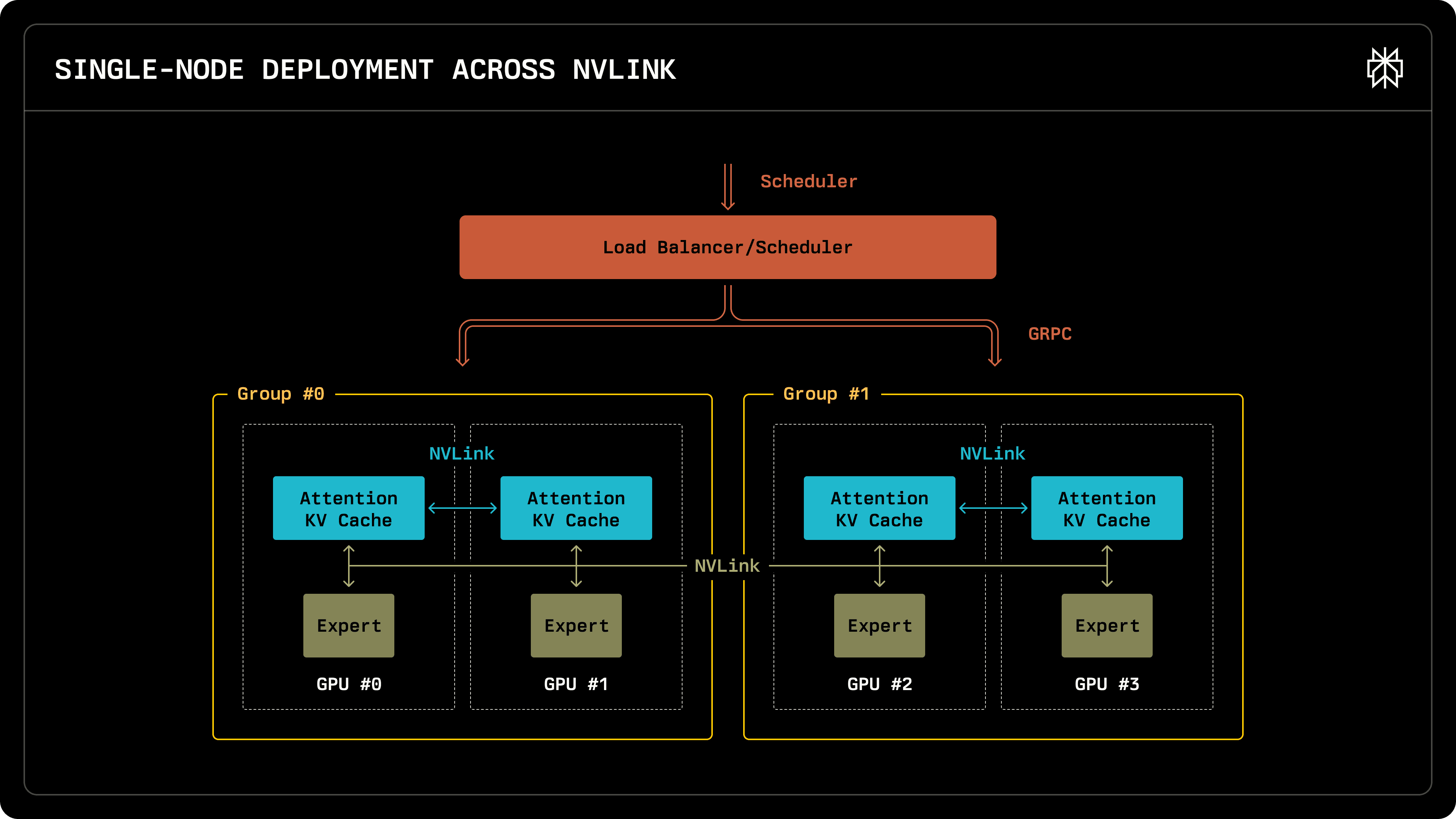
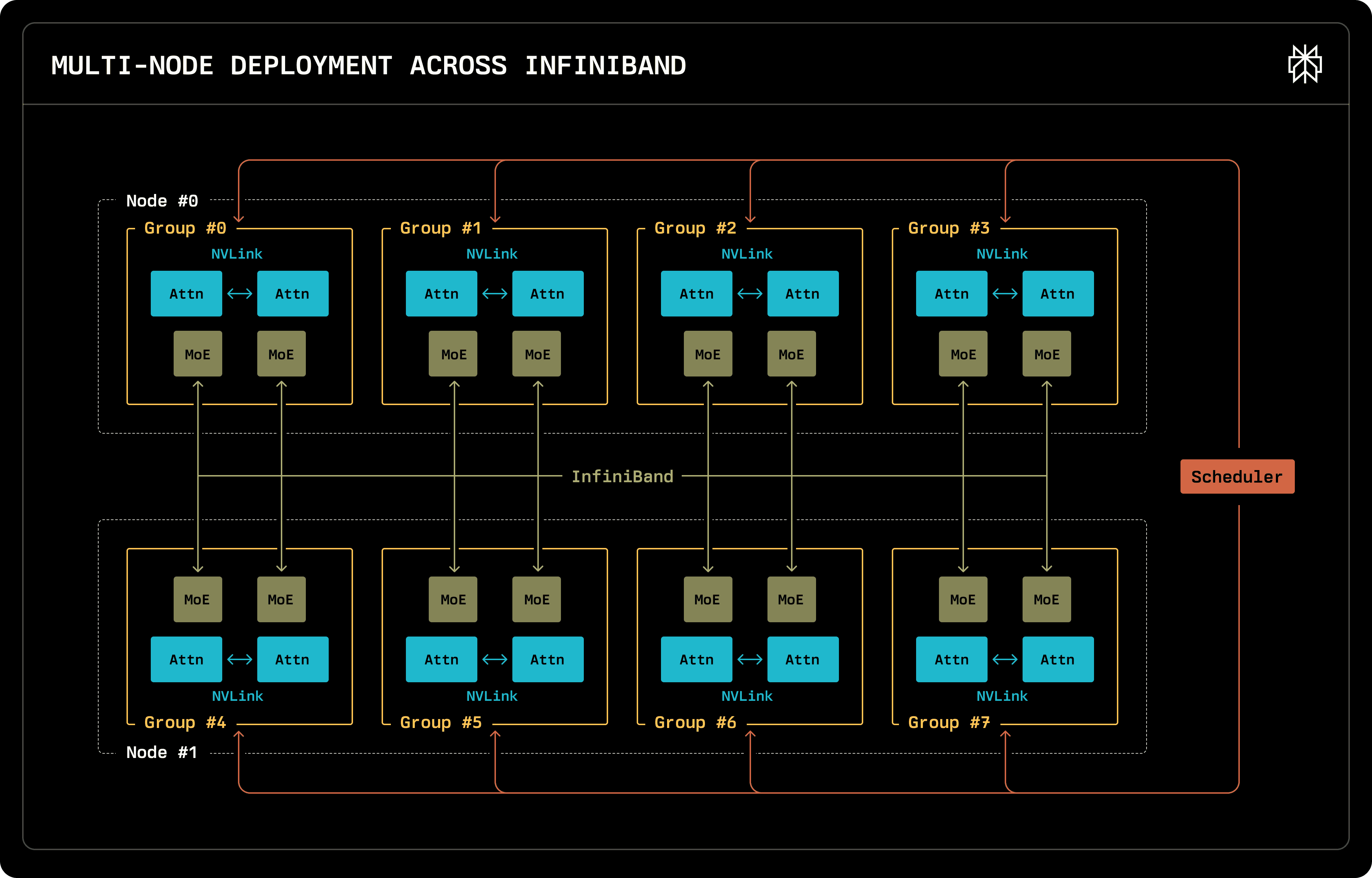
Both deployment architectures leverage Data Parallelism, orchestrated through our in-house request scheduler. Data parallelism implementation involves launching multiple inference engine instances, each operating independently to serve and maintain requests. The request scheduler, which interacts with the engine through GRPC, is responsible for spreading out requests as evenly as possible, while also facilitating KV re-use, sending requests with partial matched prefix to the servers containing the cache. Engine instances do not span multiple nodes. They can optionally use tensor parallelism to shard attention across multiple devices. The instances are inter-connected via NVLink in the single-node case or InfiniBand for the multi-node case, dispatching and collecting experts.
The single-node deployment configuration delivers superior latency with small batch sizes; however, performance degrades rapidly under increased load conditions.
To deploy the serving engine, we launch one pod per node hosting multiple engine instances. PyTorch is responsible for setting up the distributed communication and negotiating the NVSHMEM initialization. For communication, we rely on custom CUDA kernels described in an earlier blog post. The implementation of the two deployments is virtually identical, with the model picking the correct kernels to use based on the fabric implementing expert parallelism.
Parallelization Techniques
Before diving into our performance comparisons, it's essential to understand the key parallelization strategies that make deploying massive MoE models like DeepSeek-V3/R1 possible.
Tensor Parallelism
In LLM inference, Tensor Parallelism (TP) is typically used to reduce memory usage and computation per GPU, thereby reducing latency. Usually, we can shard Linear Projections in Attention and MLP Layers along row or column dimensions, and shard Attention operations along the attention head dimension.
With TP, Llama-3 architecture has no duplicated computation for Linear Projection and Attention operations across GPUs, which is an ideal sharding method. However, in DeepSeek-V3/R1 models, TP cannot achieve this.
DeepSeek-V3/R1 models use Multi-Latent Attention (MLA). An MLA Layer first uses a Linear Projection kv_a_proj to compute the latent vector, then uses another Linear Projection kv_b_proj to transform it into the space of each attention head. Since all attention heads share the same latent vector, TP cannot shard the latent vector, so all TP Ranks need to replicate the parameters and computation of kv_a_proj and kv_b_proj. Similarly, since MLA stores the latent vector in the KV Cache, each TP Rank stores an identical copy of the KV Cache.
Despite some duplication in MLA, Tensor Parallelism still provides partial reduction in computation demands, rendering it valuable for scenarios requiring high output speeds.
Expert Parallelism
DeepSeek-V3/R1 models replace MLP Layers with MoE Layers. An MoE Layer has 256 routed experts and one shared expert. Each token is dispatched to 8 different routed experts for computation, and the results are weighted summed. Each token also computes in the shared expert, and the result is added to the result from the routed experts.
Expert Parallelism (EP) serves as the typical sharding approach for MoE Layers, with each GPU managing 256 / EP routed experts while maintaining a copy of the shared expert. Compared to TP, the advantage of EP is that it can distribute computation across more GPUs, reducing the computation and memory usage per GPU.
Before performing expert computation, all GPUs need to perform an AllToAll communication to dispatch tokens to the GPUs where the corresponding experts are located; after expert computation, another AllToAll communication is needed to collect computation results from various GPUs and perform weighted summation. We implemented an optimized version of these two AllToAll communication Kernels, Dispatch and Combine, using NVSHMEM. In our previous blog post, we detailed the implementation, and our kernels have been open-sourced on GitHub.
Data Parallelism
With EP, we can distribute MoE computation across 128 or even more GPUs. However, MLA computation cannot be partitioned with EP. At this point, we can introduce Data Parallelism (DP). Each DP Group has a complete copy of MLA Layer. Each DP Group accepts different inputs and performs MLA Layer computation independently.
MLA layer's DP and TP can be combined, with one DP Group being split into multiple TP Ranks. MoE layer's EP can be combined with MLA Layer's DP/TP. EP = DP * TP. For example, on 16 machines, EP128 DP32 TP4 means distributing routed experts across 128 GPUs, with every 4 GPUs forming a DP Group, for a total of 32 independent DP Groups.
Single-Node vs Multi-Node
DeepSeek's 671B parameters exceed the memory capacity of a single 8-GPU H100 machine (80 GB * 8), but a single 8-GPU H200 machine can fully accommodate the entire model (141 GB * 8). Using the EP8 DP8 TP1 configuration, the model uses about 100 GB of memory per GPU, leaving approximately 40 GB for KV Cache and other intermediate results. One token occupies 70,272 bytes of KV Cache. Assuming each request has 5,000 tokens, each GPU can accommodate roughly 100 requests.
We wanted to understand the performance differences between single-node and multi-node deployments under different configurations. We used one H200 machine for single-node deployment and up to 16 H100 machines for multi-node deployments. For each deployment environment, we used combinations of TP 1, 2, 4, 8, and batch sizes per GPU of 1, 2, 4, 8, 16, 32, 64, 128. We assumed each request had a KV Cache length of 5,000 tokens. We also assumed Multi-Token Prediction (MTP) predicts 1 additional token (i.e., each request's query length is 2), and conservatively assumed an acceptance rate of 60%. The figure below shows the throughput and output speed for different configurations.

The horizontal axis represents output speed per request in tokens/s. The vertical axis uses a logarithmic scale to show throughput per machine in tokens/s. We marked the Pareto Frontier for each EP configuration with different colored lines.
In scenarios with extremely high output speed requirements, using single-node EP8 DP1 TP8 with a batch size of 1 can achieve an output speed exceeding 100 tokens/s, but the throughput is extremely low, equivalent to the output speed. In this scenario, the entire batch has only 2 tokens, which can be dispatched to at most 2*8=16 experts, activating a total of at most 57B parameters.
In the output speed range of 80-40 tokens/s, as throughput increases, output speed decreases significantly. In contrast, EP128 has about 5x higher throughput than single-node deployment at the same output speed.
This phenomenon can be explained by examining how single-node deployments behave: increasing batch size directly correlates with an increase in activated experts. When the batch size is 1, the average number of activated experts per GPU is 2 * 8 / 8 = 2. When the batch is large enough, all experts are activated, meaning each GPU activates 256 / 8 = 32 experts. Activating more experts means the GPU needs to read more parameters from memory, significantly increasing memory bandwidth pressure. Since the decode phase of large language models is already bottlenecked by memory bandwidth rather than compute performance, increasing batch size in single-node deployment significantly reduces output speed.
Comparison of the four multi-node deployment configurations (EP16, EP32, EP64, and EP128) reveals that higher EP values shift the Pareto Frontier toward simultaneous improvements in throughput and output speed.
Using a higher EP number means each GPU is allocated fewer experts. For example, EP128 means that each GPU is responsible for 256 / 128 = 2 experts, so the memory bandwidth pressure is significantly reduced. In other words, by using a larger EP number, we effectively gain more memory bandwidth. When the per-GPU batch size is less than 64, increasing the batch size doesn't significantly affect expert computation speed because increasing the number of inputs doesn't significantly increase memory bandwidth pressure. Therefore, we observe that when using EP128, increasing batch size doesn't affect output speed as significantly.
Interestingly, on larger batch sizes (64 requests per GPU), we observed a new phenomenon: single-node deployment throughput is slightly higher than multi-node deployment. Part of the reason is that intra-node NVLink has higher bandwidth than inter-node InfiniBand. Another part is due to limitations in our implementation. We will analyze this phenomenon in more detail later.
Due to memory capacity limitations, the EP8 DP8 TP1 configuration cannot reach a batch size of 128 per GPU, so multi-node deployment is still a better choice in scenarios pursuing higher throughput.
Computation and Communication Overlapping
As briefly introduced above regarding Expert Parallelism, GPUs are idle during MoE Layer communication. To reduce waste and lower latency, we need to find data-independent computation tasks to fill this idle time.
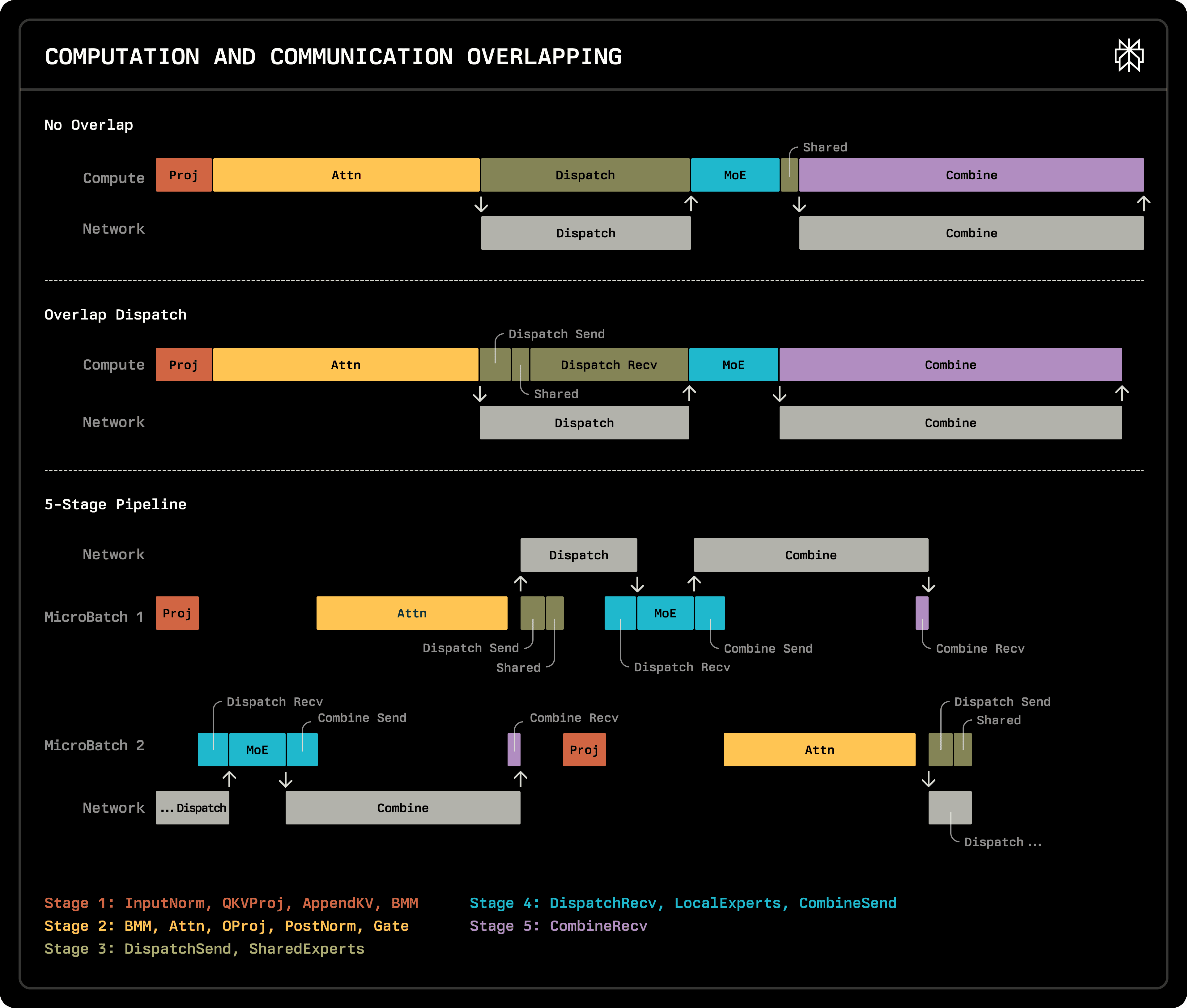
The upper part of the above figure shows the computation flow of one layer. MoE computation depends on Dispatch, and the next layer's computation depends on the result of Combine.
We place the shared expert on each GPU. This way, shared expert computation doesn't require AllToAll communication. Therefore, we can perform shared expert computation immediately after Dispatch Send, then wait for Dispatch Recv to complete. We call this overlap scheme "Dispatch Overlap".
Dispatch Overlap offers straightforward implementation and broad applicability. This technique hides shared expert computation time across all EP sizes and batch sizes.
To further increase computation and communication overlap, we used micro batching mentioned in the DeepSeek technical report to break data dependency. As shown in the lower part of the figure, we divided the computation of one Transformer Layer into 5 stages:
Stage 1: InputNorm, QKVProj, AppendKV, BMM
Stage 2: BMM, Attn, OProj, PostNorm, Gate
Stage 3: Dispatch Send, Shared Expert
Stage 4: Dispatch Recv, MoE, Combine Send
Stage 5: Combine Recv
In the first 3 Dense Transformer Layers, we use the whole batch. In the following 58 MoE Transformer Layers, we evenly divide the batch into two micro batches. The two micro batches execute alternately, offset by 3 stages. Since there is no data dependency between these two micro batches, we can switch to another micro batch's computation after Dispatch Send and after Combine Send.
Latency Breakdown
Next, we compare the effects of overlapping through an experiment, as well as compare the performance differences between single-node deployment EP8 and multi-node deployment EP128. For ease of comparison, we used H100 GPUs for the following experiment. We used TP1, a batch size of 128 per GPU, a Query length of 2 per request, and a KV Cache length of 5000.
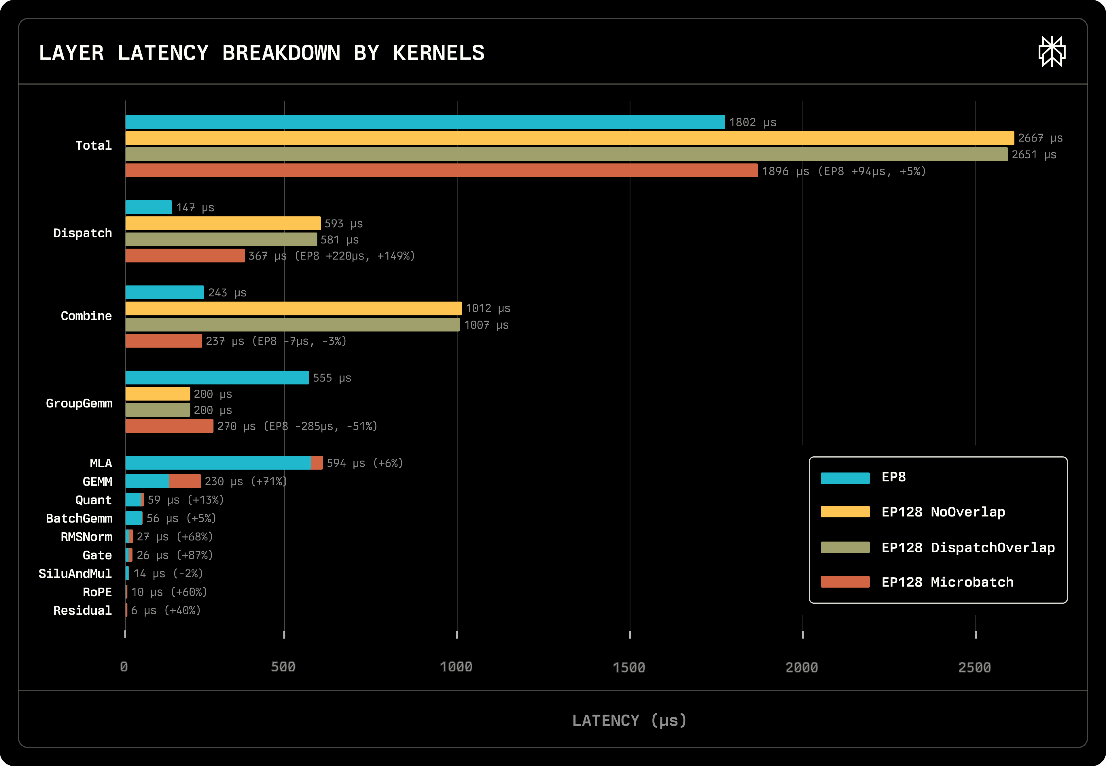
The figure above shows the total time spent on one MoE Transformer Layer and the latency proportion of different types of kernels. Except for Dispatch, Combine, and GroupGEMM, the execution time of other kernels should be equal in the EP8, EP128 NoOverlap, and EP128 DispatchOverlap series because the batch size is the same.
Overlapping
Let's first compare the effects of the three overlapping methods. NoOverlap took 2667µs in total, DispatchOverlap took 2651µs, saving 16µs or only 0.6%. MicroBatch showed a very significant improvement, taking 1896µs, a 29% speedup. Both Dispatch and Combine time were significantly reduced. Dispatch decreased from 593µs to 367µs, and Combine from 1012µs to 237µs.
Note that for computation kernels, splitting a batch of size 128 into two batches of size 64 increases the total execution time. Therefore, although the time spent on communication reduced by 1001µs, the total time only reduced by 771µs. We will explain the reason using the Roofline model in the following section.
For this reason, microbatching doesn't always improve performance.

The figure above shows the performance improvement of Microbatch compared to DispatchOverlap for batch sizes 4-128. When the batch size is less than 32, Microbatch decreases performance by 5%-40%. When the batch size is greater than or equal to 32, Microbatch can improve performance by 10%-35%.
EP8 vs EP128
Let's return to the previous figure and compare EP8 and EP128 Microbatch. EP8 took 1802µs in total, slightly less than EP128's 1896µs. Besides the increased kernel execution time brought by Microbatch mentioned above, the main differences are in GroupGEMM used for MoE computation, and the two communication kernels, Dispatch and Combine.
EP8's GroupGEMM took 555µs, while EP128's GroupGEMM took 270µs, reducing by half. This is the core advantage of multi-node deployment.
Unfortunately, the time spent on communication increased by 213µs, which greatly offset the advantage of GroupGEMM. In separate performance tests of our communication kernels, we found that they can only achieve half of the Infiniband bandwidth. We will continue to optimize our communication kernels.
Another kernel that significantly lags is GEMM. Microbatch increased GEMM by 95µs. We will analyze GEMM in more depth in the Roofline section below. We believe that the current GEMM implementation has not yet achieved optimal performance.
Roofline
The Roofline Model is a good tool for analyzing kernel performance. Its horizontal axis is Arithmetic Intensity, the ratio of FLOP to memory I/O bytes. The horizontal axis value can be calculated directly from the kernel's semantics. The vertical axis represents achieved performance, calculated by dividing FLOP by benchmark latency.
The theoretical upper bound of kernel performance is directly determined by the GPU's specifications. The H100's FP8 peak performance is 1979 TFLOP/s, represented as a horizontal line in the Roofline model. The H100's memory bandwidth is 3.35 TB/s, represented as the slope of a line passing through the origin. The two lines give the performance limits for compute-bound and memory-bound kernels, respectively.
Below, we discuss the performance of the GroupGEMM and GEMM kernels.
GroupGEMM
The GroupGEMM kernel in MoE performs the following computation: There are g groups in total, the i-th group has m_i tokens, performing a matrix multiplication of [m_i, k] x [k, n] -> [m_i, n]. In performance testing, we assume that the number of tokens in each group is the same, denoted as m_i = m. Then the FLOP count for GroupGEMM is 2 * g * m * k * n, and the memory I/O bytes is g * (m * k + n * k + m * n).
In the DeepSeek-V3/R1 model, there are 256 experts, and each token is dispatched to 8 experts for computation. Assuming a batch size of 128, query length of 2, using EP128 DP128 configuration, the average number of tokens received by each expert (i.e., m) is 128 * 2 * 8 * 128 / 256 = 1024. Similarly, we can calculate m for other configurations and batch sizes.
We used DeepGEMM's GroupGEMM implementation for performance testing. Test points covered combinations of EP8, EP16, EP32, EP64, EP128 configurations with TP1 and batch sizes 1-128.

The figure above shows the Roofline model for GroupGEMM under different EP configurations. Different EP corresponds to different numbers of groups. The figure illustrates nearly overlapping performance lines, indicating that GroupGEMM performance is predominantly determined by the total token count (represented as g * m).
The stars mark the data points corresponding to a batch size of 128 per GPU for each EP configuration. Comparing these starred data points, we can see that as EP increases (and DP increases synchronously), the number of tokens per expert m also increases. At EP8, m=128, while at EP128, m=2048.
As m increases, Arithmetic Intensity also increases. In most configurations, GroupGEMM is limited by memory bandwidth, so increasing m improves performance.
GEMM
The GEMM kernel corresponds to Linear Projections in the model, such as Q/K/V/O Projection. For a matrix multiplication of [m, k] x [k, n] -> [m, n], the FLOP count is 2 * m * k * n, and the memory I/O bytes is m * k + n * k + m * n. We can also test the latency for batch sizes 1-128.

The figure above shows the Roofline model for GEMM under different EP configurations. We can see that GEMM performance is limited by memory bandwidth. As batch size increases, Arithmetic Intensity also increases, thus improving performance.
Microbatch
When using microbatching, we divide the batch evenly into two parts. From the two figures above, we can see that when m becomes m/2, the efficiency of matrix multiplication decreases. Therefore, executing two matrix multiplications of size m/2 takes longer than executing one matrix multiplication of size m.
Multi-Token Prediction
Throughout this article, we have assumed the use of Multi-Token Prediction (MTP) for speculative decoding. MTP changes the query length per request from 1 to 2. For matrix multiplication, this is equivalent to changing m to m * 2, thereby increasing matrix multiplication efficiency. On the other hand, if we draw the Roofline model for MLA, we would find that increasing query length significantly increases MLA kernel efficiency.
Therefore, the use of MTP plays an important role in model efficiency.
Implementation & Optimizations
In this section, we will introduce some implementation and optimization details for our DeepSeek-V3/R1 model.
Quantization
DeepSeek-V3/R1 was natively trained on FP8 using a per-block quantization scheme, with weights quantized statically and activations quantized on-the-fly. Instead of computing a scaling factor per channel or per matrix statically, scaling factors are computed across 128-element vectors for activations and 128x128 element tiles for matrices, limiting accuracy degradation due to quantization.
At Perplexity, we rely on a mix of CUDA and Triton kernels to support inference, with CUDA being used for the most performance-sensitive and infrequently modified kernels (such as attention and GEMM), with Triton implementing a wide range of activation, normalization and utility kernels. Triton allowed us to quickly adapt the kernels to the block quantization scheme.
For linear and MoE layers, we mix the Deep GEMM kernels with our own Triton GEMM kernels, as we have noticed that for certain matrix dimensions and low batch sizes Split-K delivers lower latency. If the unquantized layer performs a (M, K) x (K, N) multiplication, it needs (M x ceil_div(K, 128)) x (ceil_div(K, 128), ceil_div(N, 128)) scaling factor for block quantization. For block quantization, the scaling factors for activations are computed on-the-fly, instead of being pre-calibrated. Since activation scaling factors are aggregated only along the K and not along the M dimension, kernels require only slight alterations to support the scheme.

The SiLU activation function used by DeepSeek-V3/R1 required substantial changes to support CUDA graphs, block quantization and dynamically routed token counts. Block quantization can be problematic as it introduces horizontal reductions, however the kernel already chunked activations along their hidden dimension into blocks of 1024 elements. Within one block, the tensor to be quantized was further chunked in blocks of 128 to compute the largest absolute value, with Triton generating efficient cross-warp max reductions, adding minimal overhead.
To support MoE routing under CUDA graphs, the kernels must be aware of the routing information indicating the number of tokens per expert, instead of scheduling work based on the size of the buffers which were allocated to hold the upper bound of the token counts. We cannot split the problem based on the input tensor dimensions, so we launch a fixed number of persistent kernels that read the routing information to determine how many tokens are populated and split the work of processing the activations among them dynamically.
We have already upstreamed some of our kernels to the FlashInfer project and in the future we will be open-sourcing more of our code.
MLA Layer
We use FlashInfer for MLA computation. FlashInfer supports flexible Page Table settings and extremely high performance.
We fused q_a_proj and kv_a_proj into a single qkv_a_proj. Latency decreased from 15.4 µs + 14.8 µs = 30.2 µs to 16.7 µs.
We decomposed kv_b_proj into two matrices, k_b_proj and v_b_proj. We wrote an FP8 Block Quantized BMM kernel for computations related to these two matrices.
Cuda Graph
Cuda Graph can significantly reduce kernel launching overhead, which is crucial for performance. We create a Cuda Graph for each batch size.
Before developing our AllToAll Kernel, we used torch.all_to_all_single() for AllToAll communication. This operation requires all GPUs to use the same batch size. However, different DP Groups may run different batch sizes.
To ensure all_to_all_single() is compatible with different DP Groups using different batch sizes, we first used an allreduce() operation before each model run to get the maximum batch size among all DP Groups. Then we made all DP Groups use this batch size to run.
Although this approach ensures we can use Cuda Graph, it has three disadvantages. First, it requires an additional allreduce() operation. Second, DP Groups with smaller batch sizes are forced to pad. Third, it makes our implementation code complex.
After implementing our own AllToAll Kernel, we no longer require all GPUs to use the same batch size. Therefore, we no longer need to perform additional allreduce() operations or pad batch sizes.
MoE Router
The MoE router is implemented in Triton, relying on a modified sort derived from the standard library which also keeps track of the indices of the sorted elements. The implementation is shared across all MoE models, as Mixtral routing is a special case of the DeepSeek routes where the Top-K group is the same as the group of all experts. The sparse kernels consume the Top-K indices and scores directly, whereas dense dispatch/combine schemes relying on all-to-all require routing information to be aggregated per-expert instead of a per-token basis.
Future Work
In future work, we plan to further optimize the performance of the DeepSeek model.
The most important next optimization is Prefill Disaggregation. The Prefill phase and Decode phase of the DeepSeek-V3/R1 model have very different computational characteristics. Both can use different optimization strategies and deployment schemes.
For the MLA Layer, in the Decode phase, we use Matrix Absorption to reduce the FLOP count of MLA computation. In the Prefill phase, first projecting the latent vector into K/V space and then computing in Multi-Head Attention (MHA) form would perform better.
If Prefill and Decode run on the same GPU, to reduce the impact of Prefill on Decode output speed, we typically use chunked prefill to divide the query into multiple chunks for Prefill. Because the KV Cache stores the latent vector, it becomes difficult to convert MLA into MHA form.
For the MoE Layer, in the Decode phase, we use as large EP and DP as possible to increase the number of input tokens per expert, thereby improving GroupGEMM performance. In the Prefill phase, because the number of tokens is already large enough, GroupGEMM is already compute-bound. Therefore, for Prefill, we can use smaller EP and DP.
If Prefill and Decode run on the same GPU, as long as any DP Group is performing Prefill, the latency of MoE Layers on all GPUs will increase, significantly affecting Decode output speed.
Besides Prefill Disaggregation, we also plan to optimize the following aspects:
AllToAll Performance: Our AllToAll kernel currently can only achieve 1/3 of the Infiniband bandwidth. We will continue to optimize this kernel.
EAGLE-style speculative decoding: In the data above, we assumed using speculative decoding to predict 1 token. EAGLE can use a tree structure to predict multiple tokens, improving acceptance length, which can significantly increase output speed.
GEMM Kernel: In the Roofline Model shown earlier, we can find that the efficiency of the GEMM kernel is still far from the theoretical limit. We will continue to optimize this kernel.
GB200 NVL72: In NVIDIA's latest GB200 NVL72 solution, 72 Blackwell GPUs are interconnected via high-speed NVLink. For MoE architecture models, this is a very big opportunity and challenge.
Conclusion
Multi-node deployment of DeepSeek MoE models achieves what's typically impossible with dense LLMs: simultaneously improving both throughput and latency. By distributing experts across more GPUs, we reduce memory bandwidth pressure per device, enabling faster processing and higher system throughput. Our experiments show EP128 configurations achieving up to 5x higher throughput at equivalent output speeds compared to single-node deployments.
Computation-communication overlapping techniques like micro-batching significantly reduce multi-node communication overhead, with our implementation showing up to 40% speedup. Our custom AllToAll communication kernels and optimized kernel implementations have enabled efficient deployment of the 671B parameter model.
As MoE architectures gain popularity for their capability, these deployment strategies provide valuable insights for scaling such models efficiently.